Neural Machine translation using encoder-decoder with attention

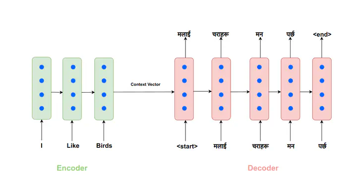
The encoder-decoder architecture consists of two components: an encoder and a decoder. The encoder processes the input sequence (for example, a sentence in the source language) and produces a fixed-length context vector, which is passed to the decoder. The decoder uses the context vector to generate the output sequence (for example, a translation of the source sentence into the target language).

fig1. English to Nepali translation using RNN-based encoder-decoder network

We discuss encoder-decoder architecture based on the example of NMT (Neural Machine Translation). NMT is a machine translation approach that uses deep learning techniques, particularly neural networks, to translate text from one language to another.

Features of encoder-decoder network

1. It can handle variable-length input and output sequences. This is because the encoder processes the input sequence and produces a fixed-length context vector, which is then passed to the decoder to generate the output sequence.
2. Encoder-decoder architecture can be trained using an end-to-end approach, where the entire model is trained to maximize the probability of the correct translation. This is in contrast to traditional machine translation systems, which typically consist of multiple separate components that are trained independently.
3. The use of RNN along with the attention mechanism can provide better results in NMT, this was the technique used before transformer-based models were introduced

The flow of the encoder-decoder network for NMT

Here is a high-level overview of how the encoder-decoder architecture works:

1. The encoder network takes in a source language sentence and converts it into a fixed-length context vector, which summarizes the meaning of the input sentence.
2. The decoder network then takes in the context vector and generates the translated output sentence, one word at a time.
3. At each step in generating the output sequence, the decoder network considers the context vector and the previous words generated as input and uses this information to predict the next word in the sequence.

Encoder and Decoder both can be understood as two simple RNNs, RNN when given the sequence of inputs produces the final output at the last time step this can be used to encode the whole sequence into a single context vector. The use of RNN as an encoder is explained in this article.

RNN as Decoder

Consider the example when a whole English sentence is passed through a single RNN and then the final output is obtained. Let’s call this the final output “context vector”. Now we can pass this context vector to another RNN but RNN takes two inputs, one is simply called input and the other is called the previous hidden state, so what do we pass as input to the RNN? we pass a special token called <start> token. This token denotes the start of the token and our Neural network will learn to start the translation when it sees this token as input.

fig2. recalling input an out of the single RNN unit

The output generated at this timestep can then be passed to the fully connected layer which has an input dimension equal to the hidden_size of the RNN unit and an output dimension equal to the vocab size. The final output vector from the fully connected layer is then passed through softmax layer, The output of the softmax layer will represent the probability of the word that is the correct word that comes after the input word. This then turns into a classification problem. we can use cross-entropy loss to train the model to output correct next word in a supervised setting.`

The full picture looks something like this

fig3. complete picture of encoder-decoder network

The advantage of the encoder-decoder is clearly depicted in the above diagram, we can encode any length sentence into a single context vector and use this single context vector to generate the translation. The translation may contain sequence of different lengths this is made possible by the above architecture because we keep on generating the sequence until we get <end> token

Information bottleneck problem

There are a few disadvantages of the encoder-decoder network like it is sequential so training these networks is slow, but the major disadvantage of the encoder-decoder network that we will talk about in this post is “information bottleneck”.

In the encoder-decoder architecture, the context vector is used to summarize the meaning of the input sequence and provide a condensed representation of the information to the decoder network. This condensed representation is often referred to as the “information bottleneck” of the model. The problem with this is that it may not be a very good approach to represent the whole sentence in this condensed manner and information from the initial part of the sequence may be lost when the sentence to be encoded is long.

Attention to the rescue

The solution to the information bottleneck problem is Attention we will discuss this briefly about the attention in this post.

fig4. decoder to encoder attention mechanism

Instead of using condensed information from the context vector, we choose to use each information encoder’s hidden state from each timestep, Attention is the mechanism in which each timestep in the decoder uses all the encoder’s hidden state to generate the next word but we also provide neural network the ability to focus differently in each of the encoder hidden state. After training the neural network with this new ability our network learns to focus on a different part of the input sentence which in turn will give a better result.

This form of attention is called encoder-decoder attention. Mathematically it is a very simple concept. we calculate the value for the attention and then use this attention value along with the decoder’s output to generate the next word.

Calculation of Attention value

1. Calculate the attention score

   Calculating the dot product between the current decoder output and all the encoder hidden states gives the attention score, This represents how much we need to focus on each token in an encoder.

2. Calculate attention distribution

   To get the probability score we pass the attention scores to the softmax function.

3. Calculate attention output

   After getting the attention distribution we calculate the weighted sum of the encoder’s hidden state weighted by the attention distribution this gives the final attention value

Prediction of the next word

The attention value is concatenated with the decoder’s output and then passed to the fully connected layer to obtain the prediction scores for the next word in an output sequence. we do this for each step in the decoder until we get <end> token.